This continues from Part 1, where we learned how the GEV distribution models extreme events and how return levels translate statistics into engineering design.
Where We Left Off
In Part 1, we discovered that extreme weather follows predictable statistical patterns (the GEV distribution), and we can calculate return levels - the intensity of events expected once every T years. This is what design codes like CSA C22.3 use when specifying "design for 50-year wind."
But here's the problem: All of this assumes the climate stays the same.
What if it doesn't?
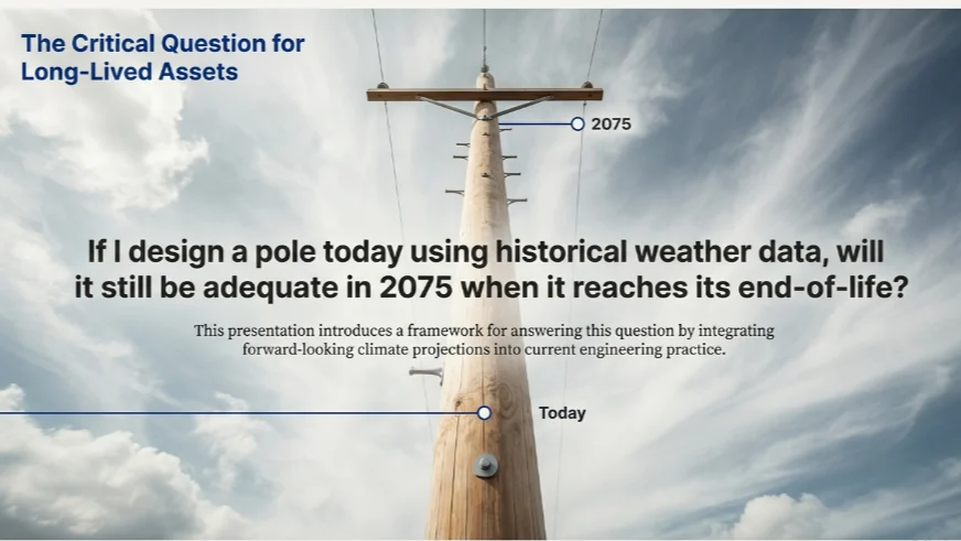
The Critical Question
"If I design a pole today using historical weather data, will it still be adequate in 2075 when the pole reaches end-of-life?"
This question leads us to a three-part framework for climate risk:
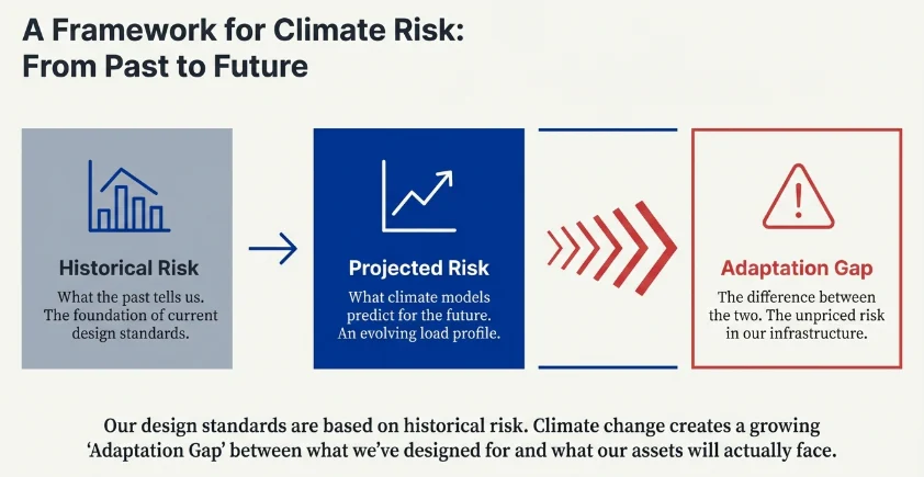
- Historical Risk — What the past tells us (what current design standards are based on; although design guidelines will have updates based on new weather data, they may not necessarily cover the extreme weather cases based on long-term climate forecasting. Engineers and designers need to fully understand the concepts behind it to make sure it fully addresses the risks)
- Projected Risk — What climate models predict for the future
- Adaptation Gap — The difference between the two (unpriced risk in current designs)
Let's walk through each part.
Step 6: Understanding "Tail Behavior" in Practice
Before we add climate projections, we need to understand something crucial: not all extremes behave the same way.
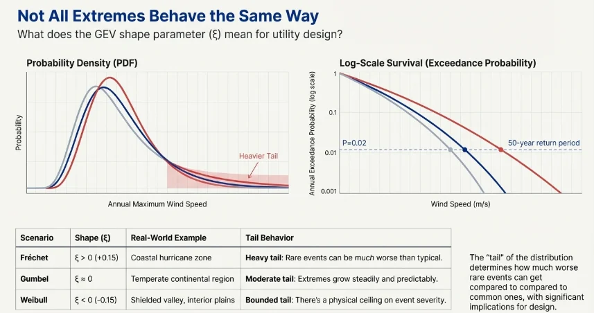
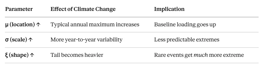
The question: We learned that the shape parameter ξ controls the "tail" of the distribution. But what does this actually mean for utility design?
The answer: It determines how much worse rare events can get compared to common ones.
Looking at the GEV Comparison Plot:
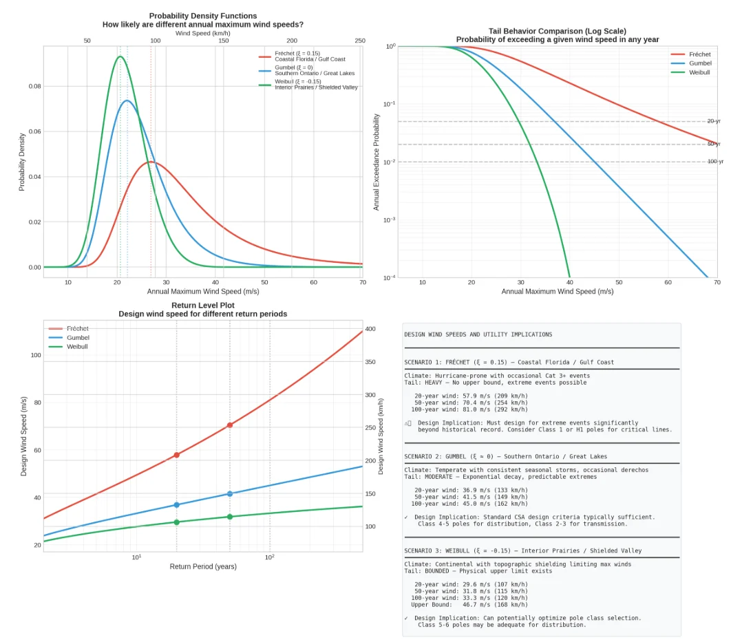
The Three Scenarios Explained:
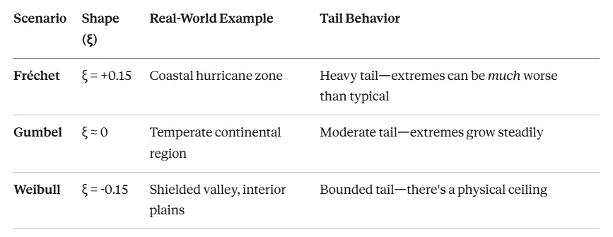
Note: IEC 60826:2017 Table D.1 confirms Gumbel distribution typically fits wind analysis well in most temperate regions.
How to Read the PDFs Plot:
The probability density shows how likely different annual maximum wind speeds are:
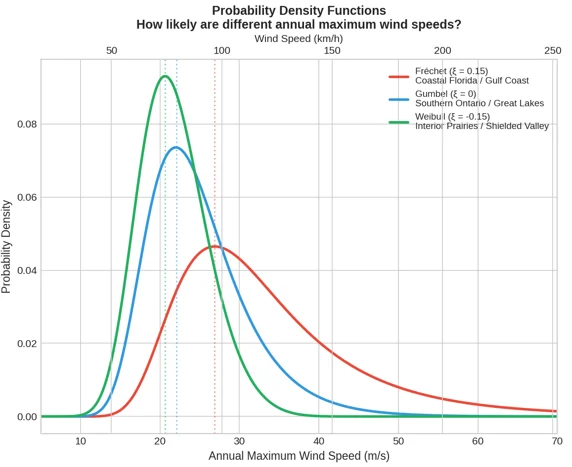
- The peak of each curve is the "most likely" annual maximum
- The right tail shows how likely very extreme events are
- The Fréchet curve extends much further right—meaning very extreme events are more probable
The Key Insight from the Log-Scale Survival Plot:
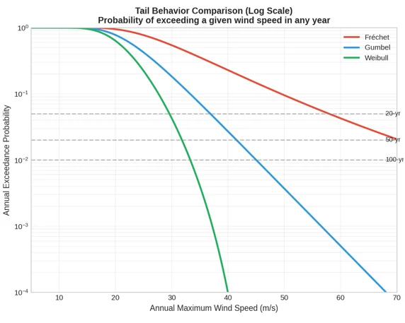
A survival plot shows exceedance probability on a log scale, with horizontal lines marking return periods:
- At the 50-year line (1/50 = 0.02 probability), read across to see the corresponding wind speed for each scenario
- The Fréchet curve hits this line at a much higher wind speed than Weibull
- This is why regions with heavy-tailed wind distributions need stronger infrastructure
Step 7: From Statistics to Pole Selection
The question: How does tail behavior translate into actual pole class decisions?
The answer: Let's work through the numbers.
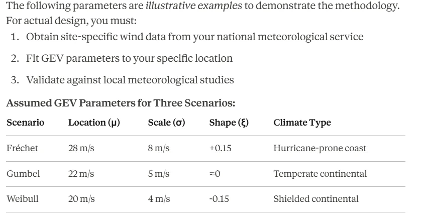
Assumptions for This Analysis:
ASSUMPTIONS — READ CAREFULLY
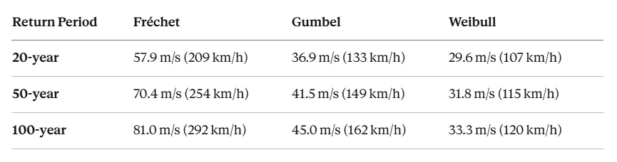
Calculated Design Wind Speeds:
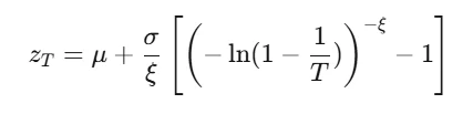
Using the return level formula from Part 1:
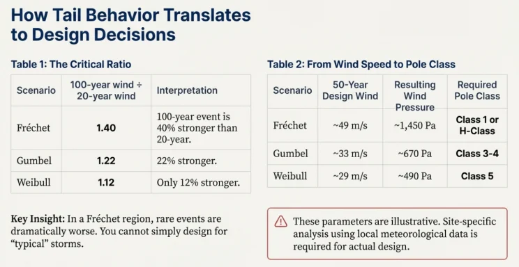
The Critical Ratio: How Much Worse Can It Get?
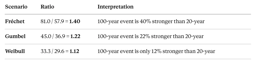
Calculate: (100-year wind) ÷ (20-year wind)
Why this matters:
In a Fréchet region (heavy tail), you can't just design for "typical" storms - the rare events are dramatically worse. In a Weibull region (bounded tail), there's less difference between common and rare extremes.
Translation to Pole Class:
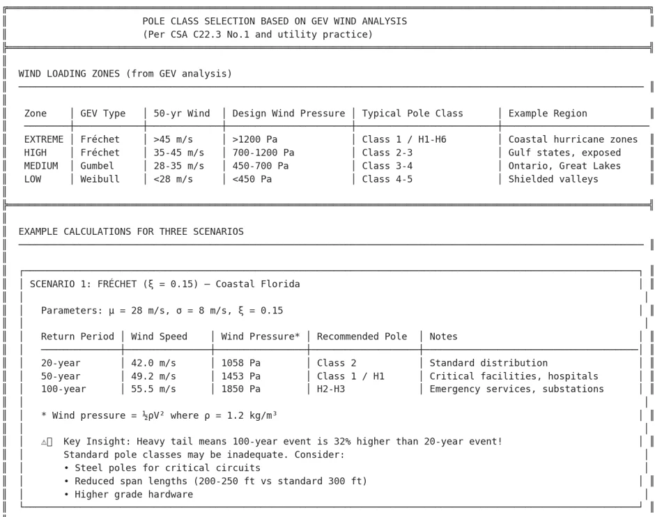
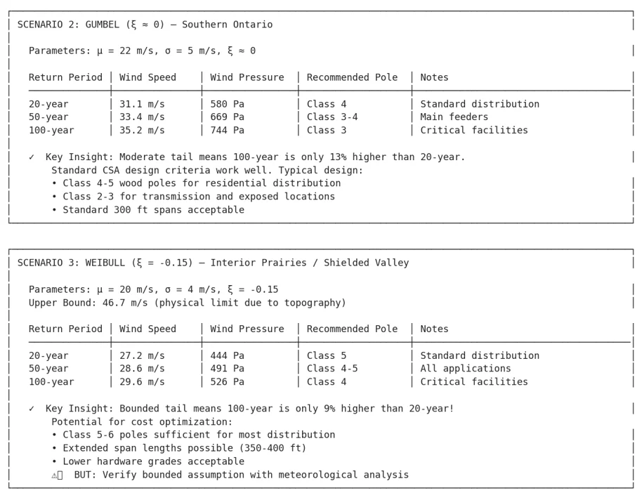
For the Gumbel scenario (temperate region):
- 50-year design wind: ~33 m/s → Wind pressure: ~670 Pa
- This corresponds to Class 3-4 poles for standard distribution
- Standard design criteria work well here
For the Fréchet scenario (hurricane coast):
- 50-year design wind: ~49 m/s → Wind pressure: ~1,450 Pa
- This requires Class 1 or H-class poles
- Standard classes are inadequate—you need premium structures
For the Weibull scenario (shielded valley):
- 50-year design wind: ~29 m/s → Wind pressure: ~490 Pa
- Class 5 poles may be sufficient
- Potential for cost optimization (but verify the bounded assumption!)
Recap:
Step 8: The Stationarity Assumption
The question: What's the hidden assumption in everything we've done so far?
The answer: We've assumed stationarity - that the climate statistics don't change over time.
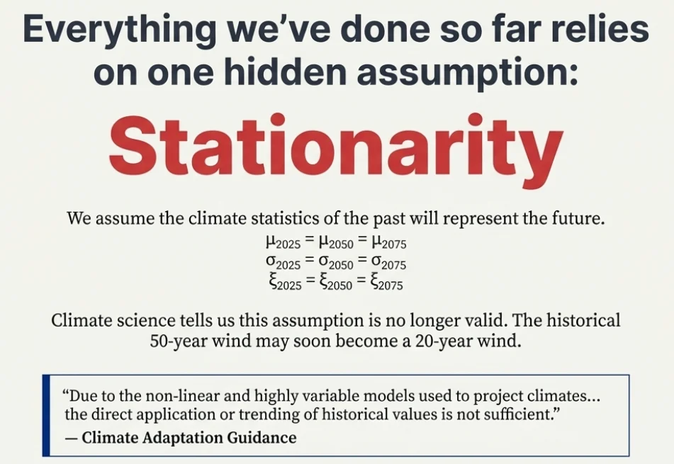
In other words: past = future.
The problem: Climate science tells us this assumption is increasingly wrong.
What Current Design Codes Do:
Design codes like CSA C22.3 specify design wind speeds based on historical weather data. When they say "50-year return period," they mean:
"Based on the past 30-50 years of weather records, this wind speed should be exceeded on average once every 50 years."
This worked fine when climate was relatively stable. But if climate is changing, the historical 50-year wind may become a 30-year wind (more frequent) or even a 20-year wind.
As climate adaptation guidance increasingly recognizes:
"Due to the non-linear and highly variable models used to project climates based on a variety of scenarios, the direct application or trending of historical values is not sufficient."
Recall this from Part 0:
The Three-Part Framework:
This leads us to separate climate risk into three components:
Step 9: Climate Projections and SSP Scenarios
The question: How do climate scientists project future extremes?
The answer: They use global climate models (GCMs) run under different emission scenarios called Shared Socioeconomic Pathways (SSPs).
The Three Main Scenarios:
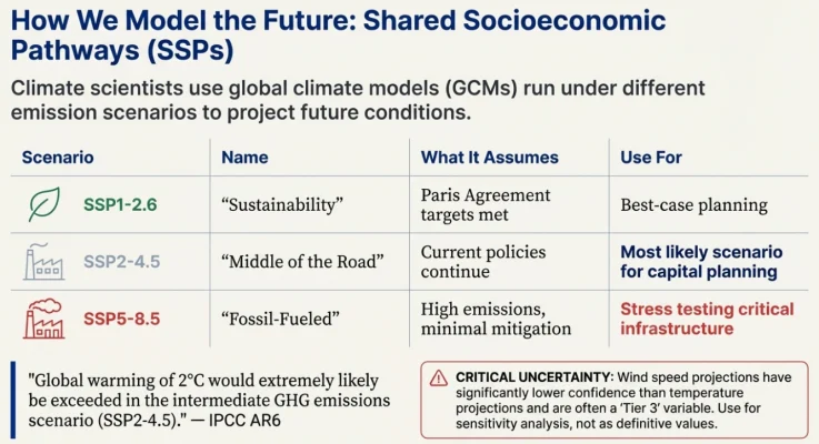
Note on RCP/SSP Correspondence: Older studies use RCP (Representative Concentration Pathway) nomenclature. The approximate correspondence is:
- RCP 4.5 ≈ SSP2-4.5 (both reach 4.5 W/m² radiative forcing by 2100)
- RCP 8.5 ≈ SSP5-8.5 (both reach 8.5 W/m² radiative forcing by 2100)
According to the IPCC AR6 Summary for Policymakers:
"Global warming of 2°C would extremely likely be exceeded in the intermediate GHG emissions scenario (SSP2-4.5)."
How Projections Affect GEV Parameters:
Climate change doesn't just shift the average—it can change all three GEV parameters.
CRITICAL UNCERTAINTY NOTE
Wind speed projections have significantly lower confidence compared to temperature projections. Government climate reports often classify design wind pressure as a "Tier 3" variable (lowest confidence tier). The projections in this document should be used for sensitivity analysis and risk awareness, not as definitive design values. Consider the possibility of both higher AND lower wind speeds than projected.
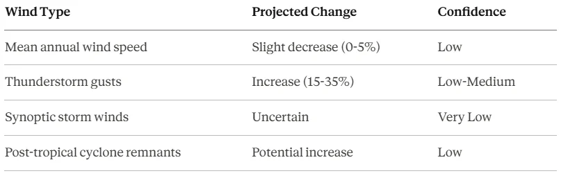
IMPORTANT NUANCE: Types of Wind Events
Climate change affects different wind phenomena differently:
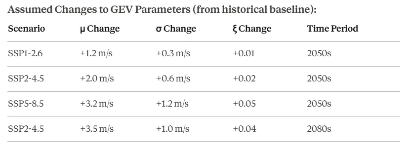
ASSUMPTIONS — Climate Projection Deltas
The following changes to GEV parameters are illustrative based on general CMIP6 trends. They are NOT derived from any specific climate model study. Actual projections require:
- Downloading specific model outputs from regional climate data portals
- Applying bias correction (e.g., Quantile Delta Mapping)
- Ensemble analysis across multiple GCMs
Step 10: Quantifying the Adaptation Gap
The question: How much stronger do we need to build if we account for climate change?
The answer: Let's calculate it for a representative temperate continental region.
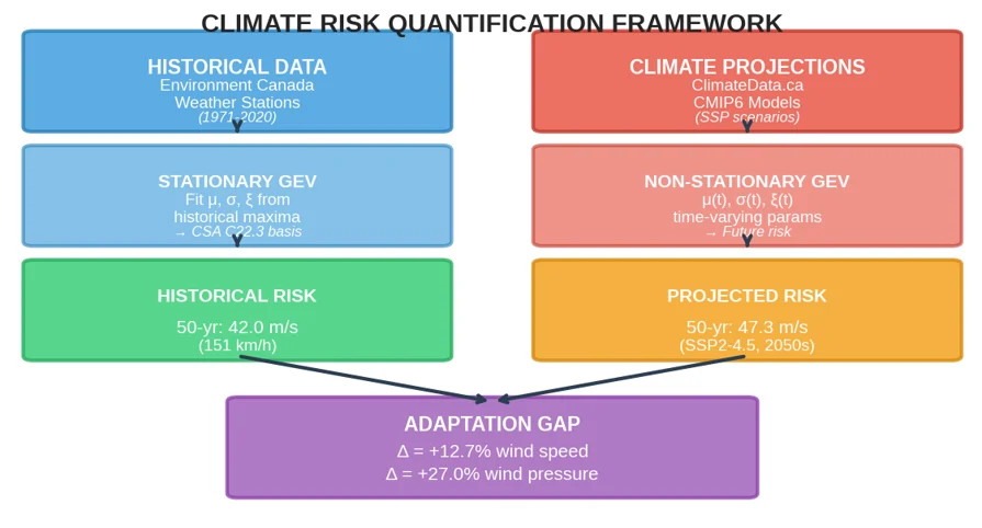
Looking at the Climate Risk Framework:
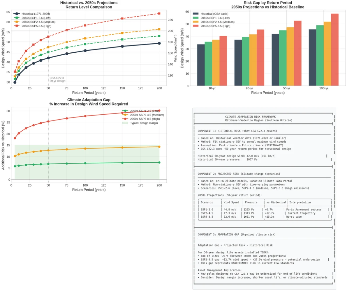
The Baseline (Historical):
Assumed Historical GEV for a Temperate Continental Region:
- μ = 22.5 m/s (typical annual maximum ~81 km/h)
- σ = 4.8 m/s (moderate variability)
- ξ = 0.02 (near-Gumbel, slight heavy tail)
For site-specific analysis, obtain parameters from your regional meteorological service using at least 30 years of annual maximum wind speed data.
Using the return level formula:
Historical 50-year design wind = 42.0 m/s (151 km/h)
This is approximately what standard design codes would prescribe for this type of region.
The Projections (2050s):
Applying the climate deltas to the GEV parameters:
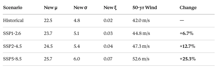
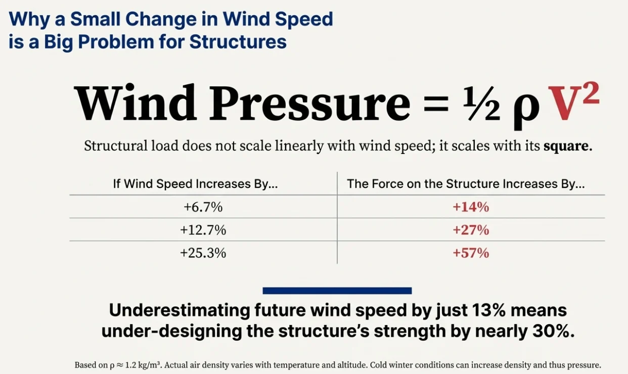
Why Wind Pressure Matters More Than Wind Speed:
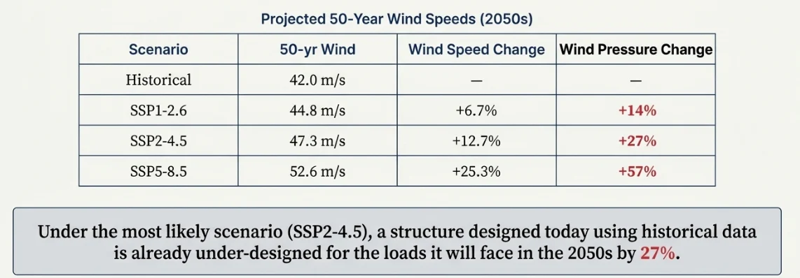
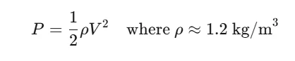
Structural loads scale with the square of wind speed:
Wind Pressure = ½ × ρ × V²
A small increase in wind speed means a larger increase in loading:
The Return Level Plot:
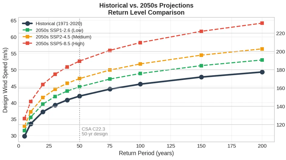
- X-axis: Return period (5 to 200 years)
- Y-axis: Design wind speed (m/s)
- Curves: Historical baseline vs. three SSP scenarios
How to read it:
- Find the 50-year return period on the x-axis
- Draw a vertical line up to each curve
- Read the corresponding wind speed on the y-axis
The vertical gap between the historical curve and the SSP2-4.5 curve represents the adaptation gap—currently unaccounted risk.
The Percentage Gap Plot:
This shows the adaptation gap as a percentage increase over historical:
- At 50-year return period, SSP2-4.5 shows ~13% additional risk
- The gap grows for longer return periods
- This is because climate change affects the shape parameter (ξ), making rare events proportionally worse
Step 11: Asset Life Alignment
The question: Does the climate when I install an asset match the climate when it fails?
The answer: Usually not - and this matters.
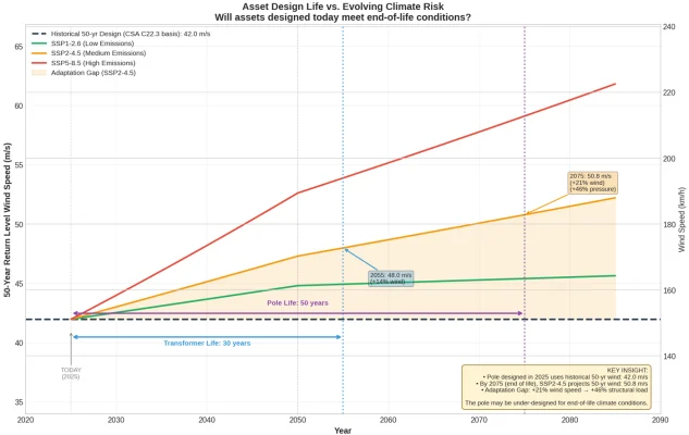
Looking at the Asset Life Alignment Plot:
The Timeline Problem:
Consider a pole installed in 2025 with a 50-year design life.
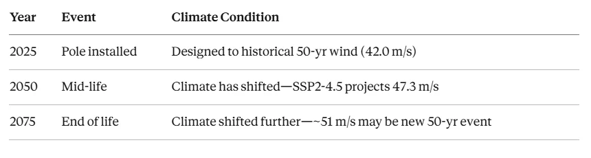
The pole was designed for a climate that no longer exists by the time it fails.
Note on Wood Pole Service Life: The 50-year design life assumption is well-established in utility practice. As the North American Wood Pole Council notes: "Depending on the environment and other factors, wood poles can last on average for some 50 years. In some locations, wood poles have remained in service for as long as 70 years or more."
Reading the Asset Life Alignment Plot:
- X-axis: Year (2025 to 2085)
- Y-axis: 50-year return level wind speed
- Horizontal dashed line: Historical design level (current code basis)
- Rising curves: SSP projections showing how the 50-yr wind evolves
- Annotated lifespans: Pole (50 years) and transformer (30 years) service periods
Key insight from the graph:
The historical design level (flat line at 42 m/s, assumed for illustration purposes) stays constant—it represents what current codes specify based on past data.
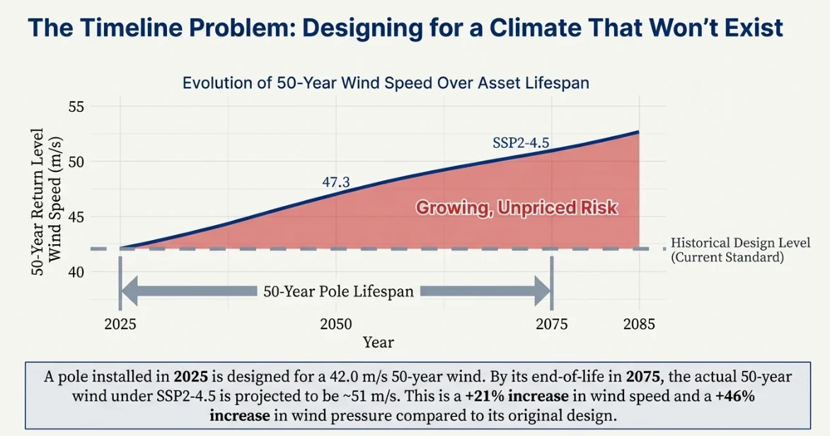
But the actual 50-year wind speed is rising (the SSP curves). By 2075:
- SSP2-4.5 projects the 50-year wind at ~51 m/s
- That's +21% wind speed and +46% wind pressure compared to design
The shaded area between the curves is the adaptation gap—the risk that's currently not priced into our infrastructure.
Step 12: What To Do About It
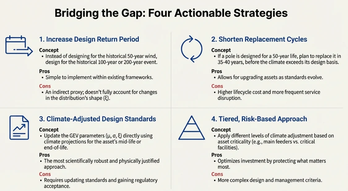
The question: If our standards are based on historical data, how do we account for climate change?
The answer: Several potential options:
The actual asset management strategy will need to be developed based on the utility's specific asset demography, geographical location, historical outage pattern with respect to weather and network model, and the overall grid modernization strategy.
The Data Sources
The question: Where does this data actually come from?
The answer: Two main sources feed the framework.
For Historical Risk
What you need:
- Minimum 30 years of hourly wind data
- Extract annual maximum for each year
- Fit GEV using Maximum Likelihood or L-moments
Note on Wind Speed Measurement Type: Wind speeds in this document refer to 10-minute mean wind speeds at 10m height in open terrain, consistent with most international standards. For gust conversion, apply appropriate gust factors (3-second gusts are typically 1.3-1.5× higher than 10-minute sustained for the same event).
For Projected Risk
What you need:
- Ensemble outputs for wind variables
- Multiple GCMs (at least 5-10 models)
- Multiple SSP scenarios for sensitivity
Note: All major climate data portals are publicly accessible without cost. Commercial alternatives may offer enhanced products for specific applications.
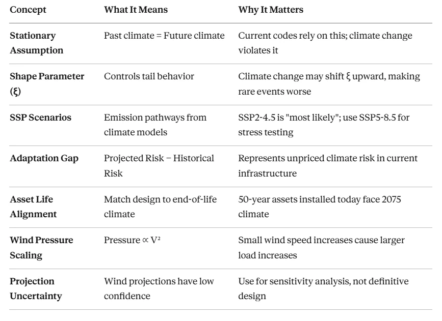
Summary: The Complete Climate Risk Framework
Key Takeaways
What's Next?
In Part 3, we'll explore:
- Multi-hazard analysis: Combining wind, ice, flood, and wildfire risks
- Fragility curves: How infrastructure damage probability relates to hazard intensity
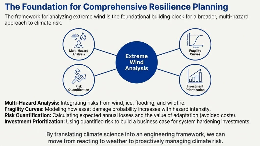
This framework provides the foundation for translating climate science into concrete engineering decisions about poles, lines, substations, and system hardening investments.
Appendix A: Formulas Reference
GEV Return Level (from Part 1):
z_T = μ − (σ/ξ)·[1 − y_p^(−ξ)]   for ξ ≠ 0
z_T = μ − σ·ln(y_p)              for ξ = 0

where y_p = −ln(1 − 1/T)
Wind Pressure:
Adaptation Gap:
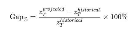
Pressure Increase:
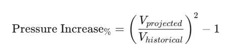
Example: If wind increases by 12.7% (from 42.0 to 47.3 m/s):

Appendix B: Suggested References
Foundational Texts
- Coles, S. (2001). An Introduction to Statistical Modeling of Extreme Values. Springer.
Standards
- CSA C22.3 No. 1 — Overhead systems
- IEC 60826:2017 — Design criteria of overhead transmission lines
- CSA S6 — Canadian Highway Bridge Design Code (includes climate adaptation provisions)
Climate Science
- IPCC AR6 Working Group I — The Physical Science Basis, 2021
- Regional climate data portals (varies by country)
Wind Studies
- Hong, H.P., Li, S.H., & Mara, T.G. (2014). Basis for recommending an update of wind velocity pressures in Canadian design codes. Canadian Journal of Civil Engineering, 41(3), 206-221.
- Cheng, C.S., Li, G., Li, Q., & Auld, H. (2012). Possible Impacts of Climate Change on Wind Gusts under Downscaled Future Climate Conditions. Journal of Climate, 25(9), 3390-3408.
Continue to Part 3: Compound Hazards and Fragility Curves.