Compound hazards and fragility curves

When Multiple Threats Strike Together

This is Part 3 of a multi-part series on Climate-Informed Asset Management for utilities. Part 0 established pole strength fundamentals. Part 1 introduced extreme value theory for single hazards. Part 2 covered climate projections and the adaptation gap. Now we tackle a harder question: what happens when hazards don't come alone?

The Starting Question

In Parts 1 and 2, we learned to model extreme wind speeds using the Generalized Extreme Value (GEV) distribution. We can now answer questions like: "What's the probability of exceeding 40 m/s wind in any given year?" or "What wind speed corresponds to a 100-year return period?"

But here's the uncomfortable reality that every utility engineer knows from experience:

The worst damage doesn't come from wind alone.

Think about the ice storms that have devastated grids across North America. The 1998 Quebec ice storm. The 2021 Texas freeze. The recurring ice events across the Great Lakes region. In each case, the damage wasn't just from ice weight - it was ice combined with wind. Conductors already heavy with ice accretion, then buffeted by moderate winds that would normally cause no concern.

Or consider the summer of 2022 in Texas, when ERCOT faced record demand. It wasn't just hot - it was hot and dry, with drought conditions reducing hydro output while heat waves drove air conditioning load through the roof.

This brings us to our central question for Part 3:

How do we model the probability of multiple hazards occurring together, and how do we translate those compound events into infrastructure damage?

Step 1: Why Independence Assumptions Fail

Let's start with a thought experiment that exposes a common mistake.

The Naive Approach

Suppose you've gone through the previous articles (Part 1 and Part 2). You know that:

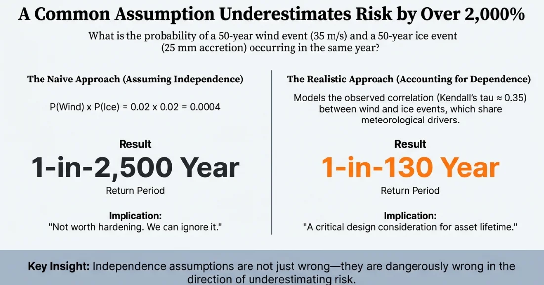
A 50-year wind event (say, 35 m/s) has a 2% annual probability
A 50-year ice event (say, 25 mm accretion) has a 2% annual probability

Common Question: "Can't I just multiply the probabilities?"

If we assume independence, the probability of both occurring in the same year would be:

P(Wind AND Ice) = P(Wind) × P(Ice) = 0.02 × 0.02 = 0.0004 = 0.04%

That's a 2,500-year return period (=1/0.04%). Sounds like we don't need to worry about it, right?

But here's the problem: these events are NOT independent.

Ice storms and wind storms share common meteorological drivers. The same low-pressure systems that bring freezing rain also bring elevated winds. The same synoptic patterns that create conditions for ice accretion often sustain those conditions with persistent wind loading.

When we look at actual historical data - 35 years of co-occurring annual maxima for wind and ice - we see a clear pattern: high wind years tend to correlate with high ice years. The observed Kendall's tau correlation is around 0.35.

The Real Probability

When we properly account for dependence using methods we'll develop in this article, that "2,500-year" event might actually be a 130-year event. That's a factor of 20x difference!

This isn't academic hairsplitting. It's the difference between:

"Not worth hardening" (2,500-year: ignore it)
"Design consideration" (130-year: consider it in planning)

Step 2: The Four Types of Compound Events

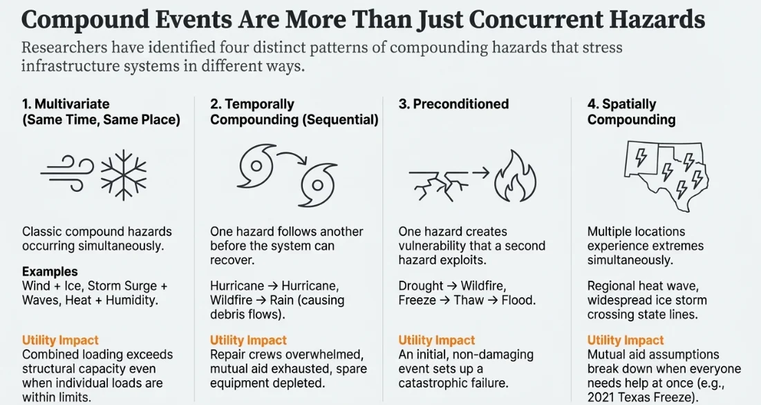
Before diving into mathematics, let's build intuition about how hazards combine. Researchers have identified four distinct patterns:

Type 1: Multivariate Events (Same Time, Same Place)

These are the classic compound hazards - two or more extremes occurring simultaneously.

Examples:

Wind + Ice: Combined loading on structures during winter storms
Storm surge + Waves: Coastal flooding during hurricanes
Heat + Humidity: Heat index extremes affecting worker safety and demand

Why it matters for utilities: Your pole was designed for either 50-year wind OR 50-year ice, not both simultaneously. The combined load can exceed structural capacity even when each individual load is within limits.

Type 2: Temporally Compounding Events (Sequential)

These are events where one hazard follows another before the system can recover.

Examples:

Flood → Flood: Second flood hits before drainage systems recover
Hurricane → Hurricane: Back-to-back storms (2017 Harvey-Irma-Maria sequence)
Wildfire → Rain: Post-fire debris flows when vegetation is gone

Why it matters for utilities: Repair crews still working on the first event when the second hits. Mutual aid exhausted. Spare equipment depleted.

Common Question: "How do we model temporal compounding?"

This requires going beyond single-year analysis. You need to look at clustering—the tendency for extreme events to occur in groups. One approach is to model the inter-arrival time between events, not just their magnitude.

Type 3: Preconditioned Events

Here, one hazard creates vulnerability that the second hazard exploits.

Examples:

Drought → Wildfire: Dry fuel loads enable fire ignition and spread
Heat → Grid stress → Blackout: Thermal limits reduce capacity, then peak demand hits
Freeze → Thaw → Flood: Frozen ground can't absorb snowmelt

Why it matters for utilities: The first event may cause no immediate damage, but it sets up catastrophic failure when the second event arrives.

Type 4: Spatially Compounding Events

Multiple locations experience extremes simultaneously, overwhelming regional response capacity.

Examples:

Regional heat wave affecting multiple utility service territories
Widespread ice storm crossing state boundaries
Coordinated wildfire outbreaks across a region

Why it matters for utilities: Mutual aid assumptions break down when everyone needs help at once. The 2021 Texas freeze affected the entire ERCOT region—there was nowhere to import power from.

Step 3: Individual Hazard Modeling with GEV (A Quick Review)

Before we can model compound hazards, we need solid models for each individual hazard. This is where Part 1's GEV distribution becomes our foundation.

The GEV Distribution

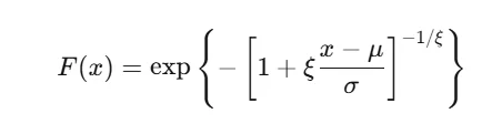
For any climate extreme (annual maximum wind, annual maximum ice thickness, etc.), the GEV distribution describes the probability distribution:

Where:

μ (mu): Location parameter — roughly the "typical" annual maximum
σ (sigma): Scale parameter — the spread of values around the location
ξ (xi): Shape parameter — controls tail behavior (how extreme the extremes get)

The corresponding probability density function (PDF) is:

Fitting GEV to Your Data

For practical application, let's consider two example hazards:

Wind Speed (Annual Maximum):

μ = 25 m/s (typical annual max)
σ = 5 m/s (variability)
ξ = 0.1 (heavy upper tail — Fréchet type)

This gives us:

50-year return level: ~38 m/s
100-year return level: ~42 m/s

Ice Accretion (Annual Maximum):

μ = 12 mm (typical annual max)
σ = 6 mm (high variability)
ξ = 0.15 (even heavier tail)

This gives us:

50-year return level: ~28 mm
100-year return level: ~32 mm

Common Question: "What if my hazard isn't well-described by GEV?"

GEV is optimal for block maxima (the maximum over fixed time blocks like years). For threshold exceedances - how often does wind exceed 25 m/s in a year, regardless of whether it's the annual max - use the Generalized Pareto Distribution (GPD). For accumulated hazards like cumulative heating degree days, other distributions may be more appropriate.

Visualizing the Marginal Distributions

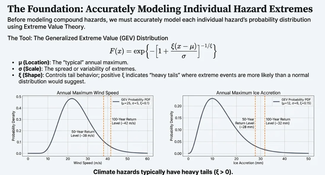
The key observation from these marginal distributions: both have positive shape parameters (ξ > 0), meaning they have heavy upper tails. Extreme values are more likely than a normal distribution would suggest. This is typical of climate hazards.

Step 4: Introducing Copulas — The Dependence Connector

Now we reach the heart of compound hazard modeling: how do we combine two (or more) GEV distributions while preserving their dependence structure?

The answer is a mathematical tool called a copula.

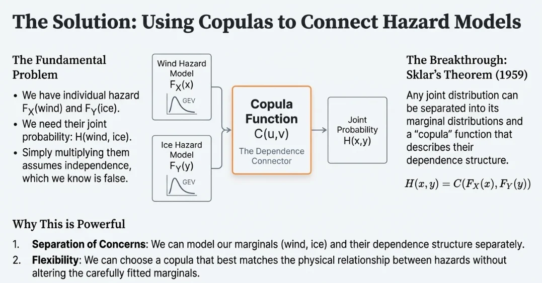
The Fundamental Problem

We have:

F_X(x): The CDF of annual max wind (our fitted GEV)
F_Y(y): The CDF of annual max ice (our fitted GEV)

We want:

H(x, y): The joint CDF — P(Wind ≤ x AND Ice ≤ y)

If wind and ice were independent:

But they're not independent. We need something that captures the correlation while respecting the fact that each marginal distribution is already well-defined.

Sklar's Theorem: The Copula Foundation

In 1959, mathematician Abe Sklar proved a remarkable theorem:

Sklar's Theorem: Any multivariate joint distribution H can be written in terms of its marginal distributions and a copula function C: H(x, y) = C(F_X(x), F_Y(y))

The copula C "couples" the marginal distributions together. It's a function that takes two uniform [0,1] variables (the probability values from each marginal) and returns a joint probability.

Why is this so powerful?

It means we can:

Fit each marginal distribution separately (wind GEV, ice GEV, heat GEV, etc.)
Choose a copula that captures the dependence structure
Combine them without changing the marginals

Recap

Common Question: "Wait, what exactly is a copula operating on?"

Let's be precise. Define:

U = F_X(X) — the "probability integral transform" of wind speed
V = F_Y(Y) — the "probability integral transform" of ice thickness

If X is drawn from its GEV distribution, then U is uniform on [0,1]. Same for V.

The copula C(u, v) tells us: "If wind is at the u-th percentile and ice is at the v-th percentile of their respective distributions, what's the probability that both are at or below those levels?"

If u = v = 0.98 (both at 98th percentile):

Under independence: C(0.98, 0.98) = 0.98 × 0.98 = 0.9604
Under strong positive dependence: C(0.98, 0.98) might be 0.98 (they move together)

Step 5: Choosing the Right Copula Family

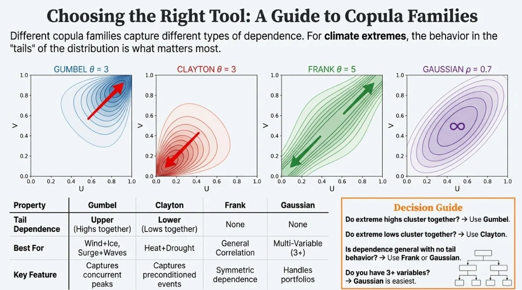
There isn't just one copula - there are many families, each with different dependence structures. The choice matters for capturing the right tail behavior.

The Major Copula Families

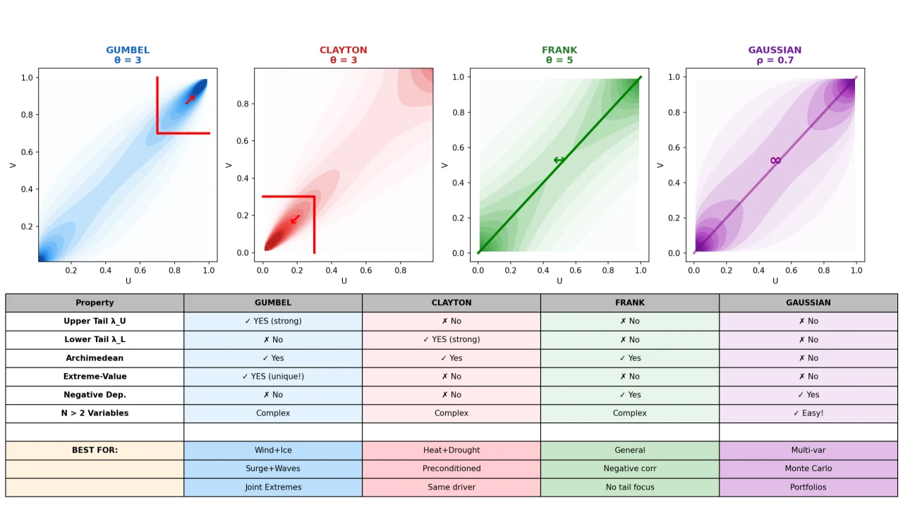
Gumbel Copula (Upper Tail Dependence)

θ ≥ 1 controls dependence strength (θ = 1 is independence); this is the dependency strength of u and v. Or, what is the chance of them appearing together.
Key property: Exhibits upper tail dependence — extreme highs tend to occur together
Best for: Wind + Ice, Storm surge + Waves — concurrent peaks during storms

The Gumbel copula is special: it's the ONLY copula that is both Archimedean (mathematically tractable) and extreme-value (appropriate for modeling joint extremes). This makes it useful for engineering modelling.

Clayton Copula (Lower Tail Dependence)

θ > 0 controls dependence (θ → 0 is independence)
Key property: Exhibits lower tail dependence — extreme lows occur together
Best for: Heat + Drought — both driven by persistent high pressure, lack of precipitation

Frank Copula (Symmetric Dependence)

θ ≠ 0 controls dependence (can be positive or negative)
Key property: No tail dependence — dependence is uniform across the distribution
Best for: General correlation without extreme co-movement

Gaussian (Normal) Copula

Based on the multivariate normal distribution. Controlled by a correlation matrix.

Key property: No tail dependence
Best for: Moderate correlations, extending to more than 2 variables

Recap in a table:

How to Choose?

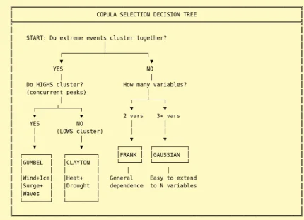
Common Question: "How do I know which copula to use for my hazards?"

Ask yourself:

Do extreme highs tend to occur together? (Both variables high at the same time)
Do extreme lows tend to occur together? (Both variables low at the same time)
Is the dependence roughly symmetric with no particular tail behavior?
Do you have enough data to test?

Step 6: Calculating Joint Return Periods

Now we can answer the practical question: What's the actual return period for compound events?

The "AND" Return Period

What's the return period for experiencing BOTH high wind AND high ice?

The annual exceedance probability for "X > x AND Y > y" is:

The return period is 1 divided by this probability.

The "OR" Return Period

What's the return period for experiencing EITHER high wind OR high ice (or both)?

Common Question: "When should I use AND vs OR?"

Use AND when you're concerned about combined loading that requires both hazards to be present (wind + ice on a conductor)
Use OR when either hazard alone causes failure, and you want to know the probability of any failure (coastal flooding from surge OR waves)

Worked Example: Wind + Ice with Gumbel Copula

Let's work through a concrete example.

Given:

Wind GEV: μ = 25, σ = 5, ξ = 0.1
Ice GEV: μ = 12, σ = 6, ξ = 0.15
Gumbel copula: θ = 2.5 (estimated from historical correlation)

Question: What's the return period for 35 m/s wind AND 25 mm ice occurring in the same year?

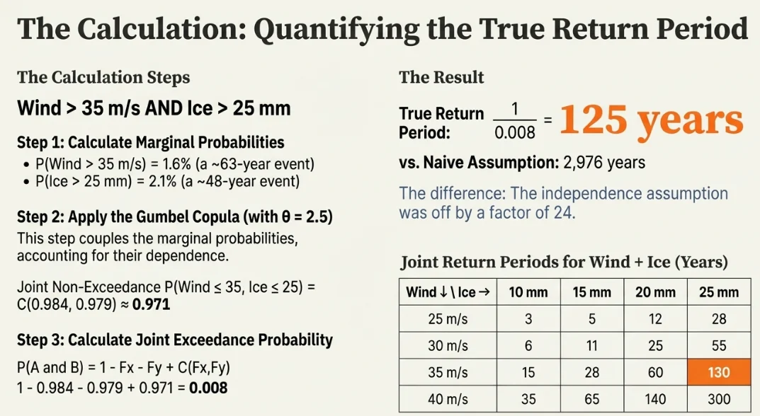
Joint Return Period Table (for illustration purposes only; construct such a table with your local data)

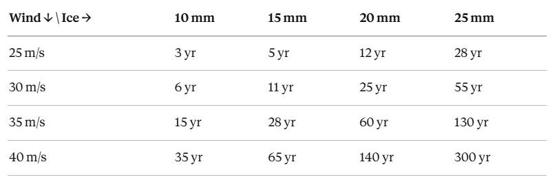
This kind of table becomes a planning tool (for illustration purposes). If your pole is designed for 50-year combined loading, you can read off what combinations of wind and ice correspond to that return period.

Step 7: Transition to Damage — Why We Need Fragility Curves

At this point, we've accomplished something important: we can calculate the probability of any combination of hazard intensities occurring (i.e., hazard occurrence).

But probability of hazard occurrence ≠ probability of damage.

A 35 m/s wind with 20 mm ice might damage some poles but not others. Why?

Material variability: Wood poles have natural strength variation (recall Part 0)
Installation quality: Some poles are set deeper, have better hardware
Decay status: A 30-year-old pole has lost capacity
Design margin: Some structures have more safety factor than required

We need a way to translate hazard intensity into damage probability → fragility curves.

What is a Fragility Curve?

A fragility curve (or fragility function) gives:

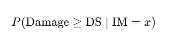
The probability that damage equals or exceeds a damage state DS, given that the intensity measure IM takes value x.

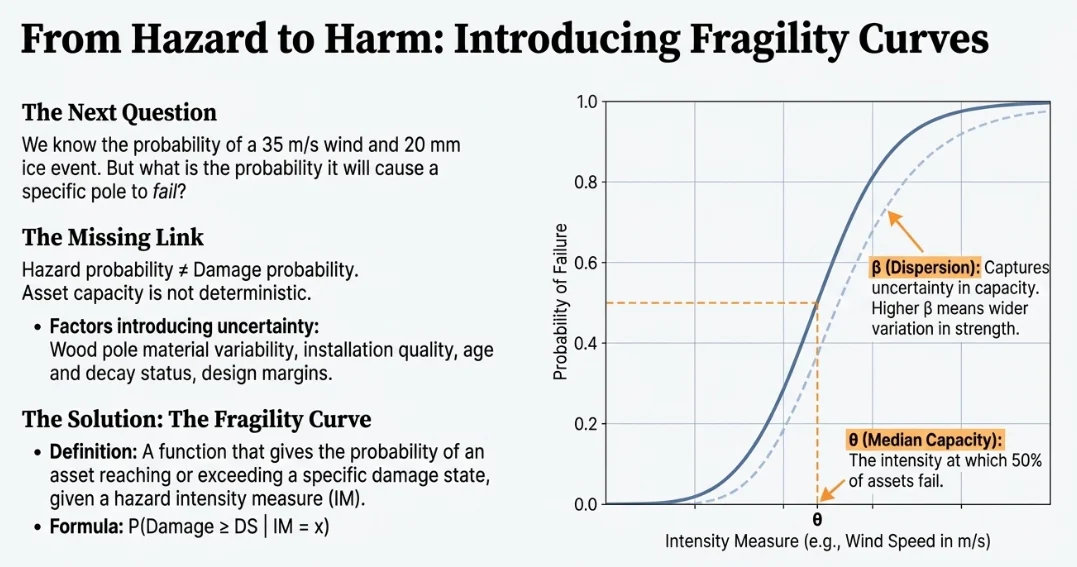
Key insight: Fragility curves capture uncertainty in capacity, not just uncertainty in loading.

Step 8: The Lognormal Fragility Model

The most common fragility formulation uses the lognormal distribution:

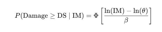
Where:

IM: Intensity measure (wind speed, combined wind+ice load, etc.)
θ (theta): Median capacity — the intensity at which 50% of assets fail
β (beta): Logarithmic standard deviation — uncertainty in capacity
Φ: Standard normal CDF

Understanding the Parameters

The Median θ:

If θ = 35 m/s for a Class 4 wood pole, then:

At 35 m/s wind: 50% of Class 4 poles would fail
Below 35 m/s: fewer than 50% fail
Above 35 m/s: more than 50% fail

The Dispersion β:

β captures "aleatory" (inherent randomness) and "epistemic" (lack of knowledge) uncertainty.

Low β (0.2-0.3): Tight capacity distribution — poles are manufactured consistently, loads are well-characterized
High β (0.5-0.6): Wide capacity distribution — older infrastructure, variable conditions, less data

Where Do Fragility Parameters Come From?

Common Question: "How do I get θ and β for my assets?"

Three approaches, in order of preference:

Empirical (Historical Failure Data)

If you have records of:

Which assets failed during past storms
What intensity those assets experienced

You can fit the lognormal fragility directly to observed failure rates. In reality, many utilities don't have enough data. The approach will be a combination of Empirical and Engineering Analysis.

Engineering Analysis (Structural Modeling)

Use structural analysis (SPIDAcalc, PLS-CADD, or similar) to:

Model a population of poles with varying properties
Apply increasing loads
Record failure points
Fit a fragility curve to the simulated results

This approach uses Monte Carlo simulation with material property distributions from Part 0.

Literature Values (Expert Judgment)

Start with published fragility parameters for similar asset classes, then calibrate to local conditions. EPRI, FEMA, and academic literature provide baseline fragility curves for common infrastructure types.

Step 9: Multiple Damage States

A binary "failed/not failed" model is often too crude. Real damage occurs on a spectrum:

Damage State Definitions for Distribution Poles

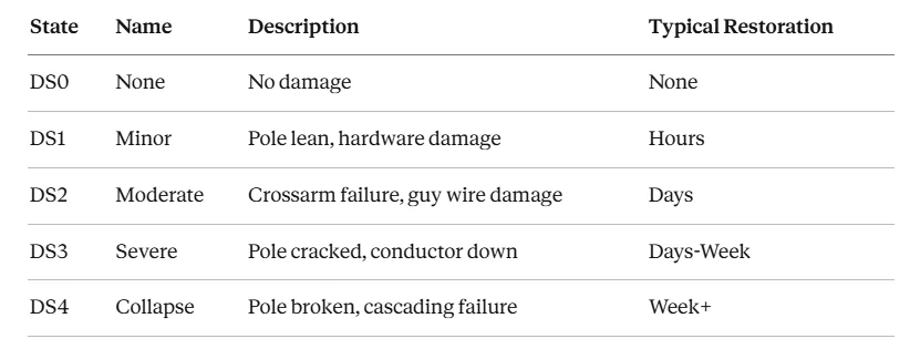
Each damage state has its own fragility curve, with progressively higher median capacities (for illustration purposes).

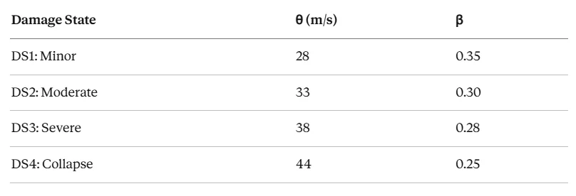
Common Question: "How do I use these for planning?"

The damage state probabilities tell you what to expect and what resources to stage:

If a 35 m/s storm is forecast: 75% of exposed poles may have at least minor damage (inspection needed); 15% may collapse (crew deployment, equipment staging)
For budgeting, multiply damage probabilities by repair costs: DS1 repair: $5,000; DS4 repair: $8,000 + cascading effects

Step 10: Multi-Hazard Fragility Surfaces

For compound hazards, a single intensity measure isn't enough. We need a fragility surface that depends on multiple inputs.

Combined Wind + Ice Loading

When ice accumulates on conductors, it affects pole loading in two ways:

Weight: Ice adds gravitational load on the pole
Drag: Ice increases conductor diameter, increasing wind drag

A common combined loading model (ASCE Manual 74):

Where:

F_wind = wind force on bare conductor
k ≈ 0.02 per mm = drag increase coefficient
t_ice = ice thickness in mm
W_ice = ice weight force

Fragility Surface for Wind + Ice

The fragility becomes a function of two variables:

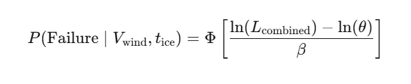
Where L_combined = f(V_wind, t_ice) from the loading model.

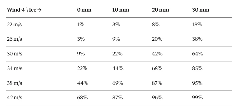
Reading the surface:

At 30 m/s wind with 0 mm ice: 9% failure probability. At 30 m/s wind with 20 mm ice: 42% failure probability.

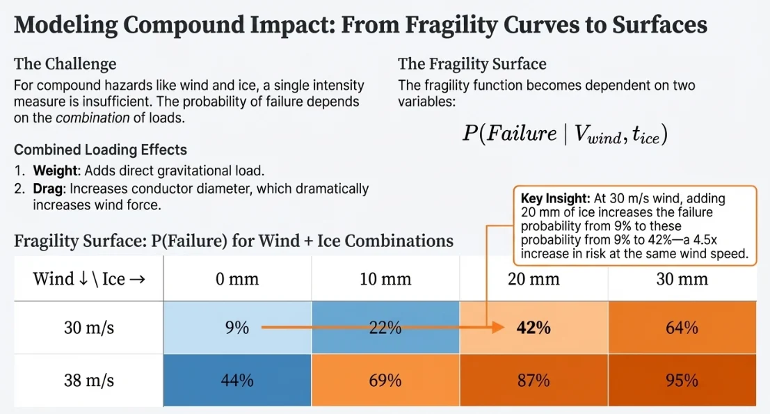
The ice more than quadrupled the failure probability, even though the wind speed didn't change!

Common Question: "Our design code already accounts for combined loading. Why do we need this?"

Design codes give you a deterministic pass/fail threshold. Fragility surfaces give you the full probability distribution. You need probabilities for:

Risk-based planning (expected damage costs) → Asset Investment Planning
Restoration planning (how many crews to stage) → Resource Dispatch for Storm
Insurance and regulatory compliance → Corporate Business Decision
Comparing hardening alternatives → Benefit and Cost Assessment

Step 11: Putting It All Together — Risk Calculation

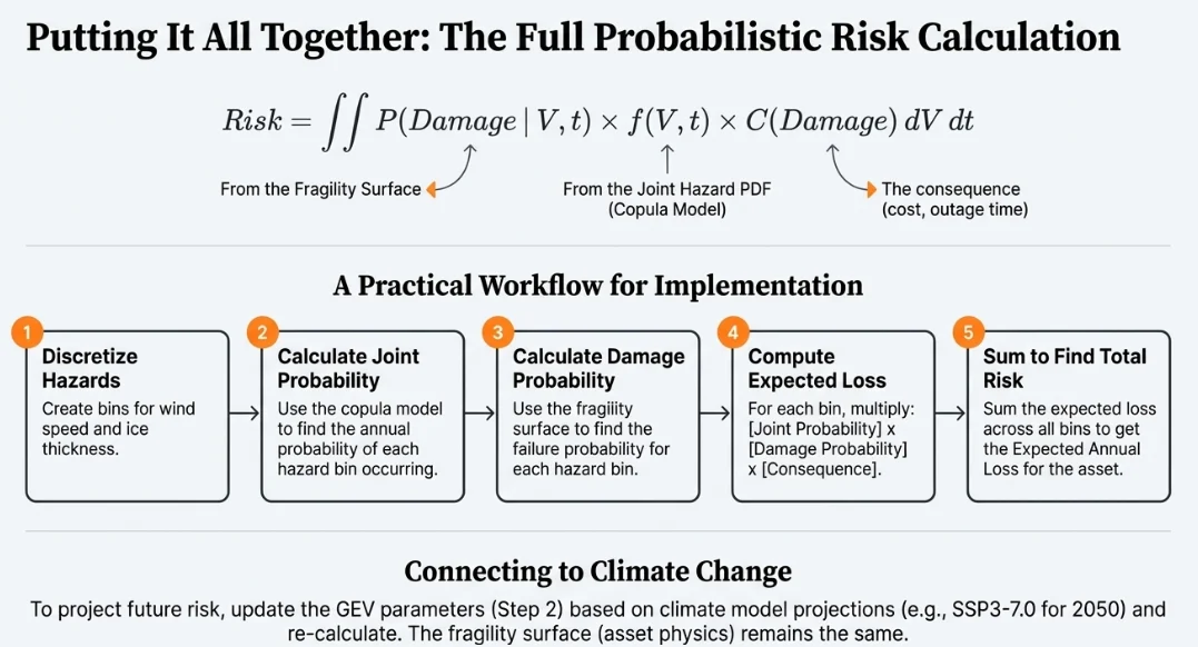
Now we can connect the pieces:

The Risk Equation

Where:

P(Damage | V, t) = fragility surface
P(V, t) = joint hazard probability from copula model
C(Damage) = consequence (repair cost, customer interruption, etc.)

Common Question: "How do fragility curves change under climate projections?"

Fragility curves typically DON'T change - they represent the physical relationship between load and capacity.

What changes is:

Hazard frequency/intensity (from climate projections)
Asset population/demography (from hardening investments)

If you upgrade poles from Class 4 to Class 2, you're shifting to a different fragility curve (higher θ), not changing the climate inputs.

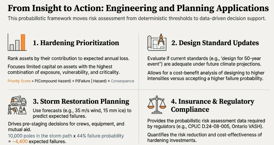
Step 12: Practical Engineering Applications

Let's connect this theory to real decisions:

Common Questions Summary

Throughout this article, we've addressed several questions that engineers frequently ask:

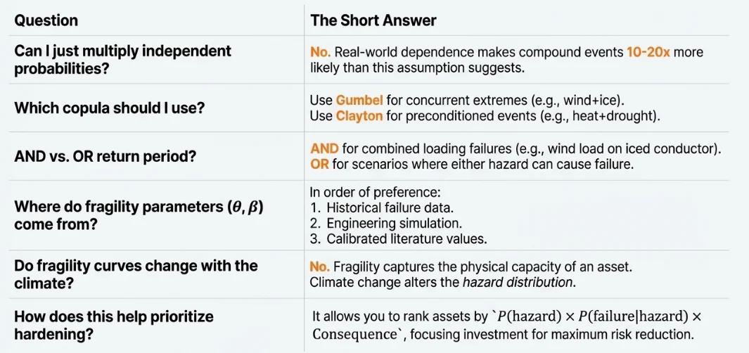
Key Takeaways

Independence assumptions fail catastrophically for compound hazards. Use copulas to model dependence.
Copula choice matters: Gumbel for upper-tail dependence (concurrent peaks), Clayton for lower-tail (preconditioned events).
Fragility curves translate hazard to damage using lognormal functions with median capacity (θ) and dispersion (β). Note: Utility data limitation warning. Often, there is not enough data to develop the fragility curves (a.k.a. failure curves); trial and error is required for fitting with both empirical data and engineering analysis.
Multi-hazard requires fragility surfaces, not just curves — damage probability depends on the combination.
Climate change shifts the hazard distribution, not the fragility relationship. Both matter for risk projection.
Practical applications include hardening prioritization, design standard updates, restoration planning, and regulatory compliance.

References

Standards & Codes

NESC C2-2023, Rule 250C/D — Combined ice and wind loading
ASCE Manual 74 (4th ed.) — Guidelines for Electrical Transmission Line Structural Loading
IEC 60826:2017 — Design criteria of overhead transmission lines
CSA C22.3 No. 1 — Overhead systems

Key Research Papers

Sklar, A. (1959). "Fonctions de répartition à n dimensions et leurs marges." Publications de l'Institut Statistique de l'Université de Paris, 8, 229-231.
Zscheischler, J., et al. (2018). "Future climate risk from compound events." Nature Climate Change, 8, 469-477.
Zscheischler, J., et al. (2020). "A typology of compound weather and climate events." Nature Reviews Earth & Environment, 1, 333-347.
Bevacqua, E., et al. (2019). "Higher probability of compound flooding from precipitation and storm surge in Europe under anthropogenic climate change." Science Advances, 5(9).
Fu, X., et al. (2019). "Fragility Analysis of Transmission Towers Subjected to Downburst Winds." Journal of Performance of Constructed Facilities, 33(4).
Khansefid, A., et al. (2025). "Multi-hazard fragility surfaces for power transmission towers." Engineering Structures.

Industry & Regulatory

EPRI (2024). "Compound Hazards and The Power Sector in a Changing Climate." Report 3002030518.
EPRI (2024). "Climate Data Users Guide." Report 3002028078.
CPUC D.24-08-005 (August 2024). Climate Adaptation Vulnerability Assessment guidelines.
Ontario Energy Board (2024). Vulnerability Assessment and System Hardening (VASH) Framework Report.

Continue to Part 4: Exposure Analysis.